Earthquake Music
by Zhigang Peng
This webpage contains earthquake "sounds" created from seismic recordings all around the world. They provide a unique way for us to listen to the vibration of the Earth that is otherwise inaudible to us, and to decipher the complicated earthquake physics and triggering processes.
Note: The material developed in this website is partially supported by the National Science Foundation's CAREER program EAR-0956051 .
I have been working closely with David Simpson, the IRIS president, and Debi Kilb, a researcher at UCSD on this topic. If you would like to use these sound tracks, I would appreciate if you could put proper acklowledgement and cite the following publication: Kilb, D., Z. Peng, D. Simpson, A. Michael and M. Fisher* (2012), Listen, watch, learn: SeisSound video products, Seismol. Res. Lett., 83(2), 281-286, doi: 10.1785/gssrl.83.2.281.
- The 2004 Mw6.0 Parkfield earthquake and its aftershock sequences are recorded
by many near-field instruments on scale. The following plot shows the vertical component
seismogram recorded by one of the SAFOD Pilehole instrument. The top panel shows the raw data.
The middle panel is the spectrogram, which shows the mainshock and numerious aftershocks in
the first 1000 s immediately after the mainshock. The bottom panel is 40 Hz high-pass-filtered
envelope function. The blue lines correspond to events listed in the NCSN catalog, while the
red lines represent events identified by a waveform matched filter technique (Peng and Zhao,
Nature Geosci., in review, 2009). By directly listening to the sound track below, you could also hear clearly
the mainshock and distinct early aftershock signals.
-

-
- pkfpilot_16x_10.wav sped up 16x, amplitude divided by 10, will clip (created by Andy Michael and Bill Ellsworth, downloaded from the following website: 09/28/2004 - Sounds of the Parkfield earthquake
- Detection_Plot1.mov Animations of newly detected aftershocks in the first hour
after the 2004 Mw6.0 Parkfield earthquake (Peng and Zhao, Nature Geosci., 2009).
- On 2008/05/12, the disastrous Mw7.9 Wenchuan earthquake ruptured ~250 km along the Longmenshan thrust belt along the Longmenshan
thrust belt that bounds the Tibetan plateau and the Sichuan basin [Burchfiel et al., GSA, 2008; Xu et al., Geology, 2009]. This earthquake
and its subsequent aftershocks were recorded continuously by many permanent and temporary broadband seismometers in Sichuan and elsewhere
in the world. The following example is generated by the seismogram recorded at a nearby station CB.CD2. The mainshock signal is
clipped, but most of the early aftershock signals are not. Many of them were not listed in the standard earthquake catalog. I will be working
with scientists at China Earthquake Administration (CEA) to detect and locate these missing early aftershocks, and use them to better
understand the physics of aftershock triggering.
-

-
- CB.CD2.BHZ.SAC.wav Earthquake sound of the Mw7.9 Wenzhuan earthquake sequence in China on 2008/05/12
- Below is the image and sound of the seismic recording at station HVSC (more than 1.5 g vertical acceleration) for the 2011/02/21 Mw6.3 New Zealand earthquake. This vertical seismogram is recorded by strong motion sensors only about 1 km distance from the epicenter. From the sound below, you can hear not only the mainshock like a train running towards you, but also many small pops that are early aftershocks immediately afterward. The data can be downloaded from the Center for Engineering Strong Motion Data website .
-

-
- NZHVSC_Z.wav earthquake sound of the 2011/02/21 Mw6.3 New Zealand earthquake (speed up 20 times, amplitude slightly clipped)
- The following example shows non-volcanic tremor in central California triggered by the 2004 Mw9.2 Sumatra earthquake ( Ghosh et al., JGR, 2009 ). The triggered tremor lasted for more than 2 hours, starting during the teleseismic P waves. The following figure shows the stacked
spectrogram of 19 borehole HRSN channels with high signal-to-noise
ratio (Taken from Figure 6 of the Ghosh et al., 2009 paper). Surface wave-triggered tremor energy is observed after ~3000s. Tremor triggered
by the body waves is seen at around 1700s, when energy extends up to 15 Hz and beyond, similar to the tremor triggered by the surface waves. Note that energy up to 15 Hz and beyond can only be seen during tremors and local/regional earthquakes. The spike of strong energy at ~11000 s is an ordinary [local] earthquake. (Of course, you could also describe the sound as thunder [distance eq], followed by the rain [triggered tremor], and finally a gun shot [local earthquake]).
-

-
- Sumatra_BP.GHIB.DP1.SAC.wav (sped up 200x, amplitude normalized by 1.2*max amp)
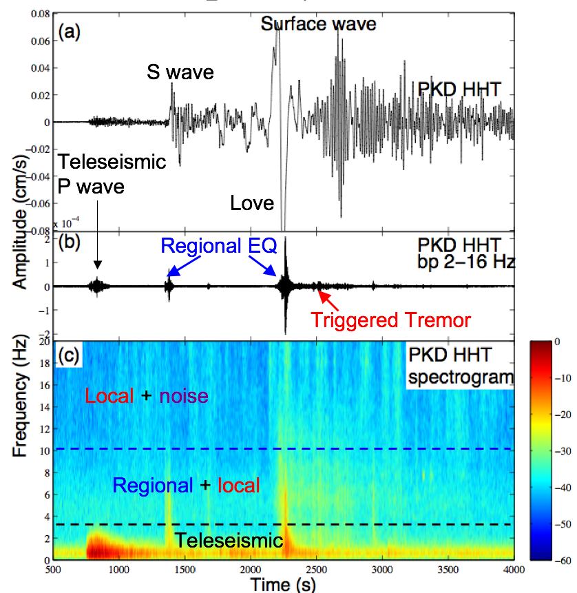
- The following example shows triggered earthquakes in the Coso geothermal area and non-volcanic tremor near the Parkfield-Cholame section of the San Andreas fault triggered by the 2010 Mw8.8 Chile earthquake ( Peng et al., GRL, 2010 ).
Several microearthquakes near the Coso geothermal field were triggered during the wavetrains from the Chilean mainshock, with the largest earthquake (M=3.4) occurred during the large-amplitude Love waves. The Chilean mainshock also triggered numerous tremor near the Parkfield-Cholame section of the San Andreas fault. The locally triggered tremor during the Love waves are masked by the regional seismic signals from the Coso region, and could only be identified after a high-pass-filter. In this audio, you can hear the P wave of the Chile mainshock as low-pitch thunder, triggered earthquakes in the Coso region as distinct gunshots, and triggered tremor around the San Andreas fault as rattle snakes. The image is generated from the instrument-corrected broadband stations PKD, while the sounds are converted from the HRSN station VCAB.
-
 -
- The seismogram shown below is recored near Mt. St Helens during the volcanic eruption in 2004. The earthquakes
occurred during this episode occurred so regularly that they are often called "the drumbeat earthquakes". It was
suggested that those nearly periodic shallow events are generated by stick-slip extrusion of a solid dacite plug
forced by magma below ( Iverson et al. Nature, 2006).
-

-
- Msh21BHZ_x300_0.5to15_new.wav (generated by Debi Kilb)
- The seismograms shown below correspond to an ambient non-volcanic tremor on 2007/05/08 near Cholame, California (per. comm. Robert Nadeau).
The tremor started at -500 s, and continuously ratted for about 1000 s. The sound below is generated from the station GHIB, which belongs to
the High-Resolution Seismic Network (HRSN) operated by UC Berkeley.
Distinct rapid-fire events could be identified within the tremor, which
may correspond to individual low-frequency earthquakes that is recently observed in this region ( Shelly, Nature, 2010 ).
-

-
- The following sound/video shows increasing amplitudes of seismic waves for three nuclear explosions in North Korea recorded at station MDJ in China. The seismic data is distributed by the Incorporated Research Institutions for Seismology's Data Management Center (IRIS DMC, IC network ).
-

-
- North_Korea_Nuke_comparison.mov (2 MB)
- The following sound/video shows seismic signals associated with the 2013/02/15 Russian Meteor Impact and recorded at station II.ARU about 230 km away. The seismic data is distributed by the Incorporated Research Institutions for Seismology's Data Management Center (IRIS DMC, II/GSN network ).
-

-
- 20130215_Meteor_Explosion.mov (3 MB)
- The following static image shows seismic waves recorded at up to 2000 km from the the Russia meteor explosion. The seismic waves are likely induced by the atmospheric shock waves, and are traveled at a speed of about 3-3.5 km/s, similar to the surface waves generated by earthquakes.
-

- The following sound shows infrasound signals associated with the 2013/02/15 Russian Meteor Impact and recorded at station TA.Y52A about 9600 km away in Lilburn, Georgia. The sound took about 10 hours to travel from Russia to Georgia. The seismic data is distributed by the Incorporated Research Institutions for Seismology's Data Management Center (IRIS DMC, TA/USArray network ).
-

-
- 20130215_Meteor_Explosion_Infrasound.mov (6.3 MB)
- The following static image shows infrasound waves recorded at up to 10000 km in Georgia and Florida from the the Russia meteor explosion. The infrasound waves are likely induced by the atmospheric shock waves, and are traveled at a velocity close to the sound speed.
-

- The following animation shows a comparison among the 2013/02/12 North Korea nuclear explosion, an M5.1 earthquake in Nevada on 2013/02/13, and the meteor impact on 2013/02/15 recorded at seismic stations a few hundred kilometers away. The initial sound of the nuclear explosion is much stronger, likely due to efficient generation of compressional wave (P wave) for an explosive source. In comparison, the earthquake generated stronger shear waves that arrived later than the P wave. Finally, the seismic signal from the meteor impact is relatively small, even after being amplified by 10 times. This is likely caused by the poor coupling between the atmosphere and solid earth.
The seismic data is is recorded at station IC.MDJ, BK.SAO and II.ARU, respectively, and is freely distributed by the Incorporated Research Institutions for Seismology's Data Management Center ( IRIS DMC ).
-

-
- Comparison_Nuclear_EQ_Meteor.mov (2.8 MB)
- The following animation shows a comparison between the 2013/02/12 North Korea nuclear explosion, and an M5.1 earthquake in Nevada on 2013/02/13. The initial sound of the nuclear explosion is much stronger, likely due to efficient generation of compressional wave (P wave) for an explosive source. In comparison, the earthquake generated stronger shear waves that arrived later than the P wave. The seismic data is is recorded at station IC.MDJ and BK.SAO respectively, and is freely distributed by the Incorporated Research Institutions for Seismology's Data Management Center ( IRIS DMC ).
-

-
- Comparison_Nuclear_EQ_Meteor.mov (2.1 MB)
- Below is a sample matlab script that can be used to convert the seismic data in SAC format to .WAV format.
This simple matlab script requires the fget_sac.m subroutine, which is in the MatSAC package . For more information about how to use the fget_sac.m, please visit
my SAC tutorial .
- Matlab code sac2wav.m .
- Example input SAC file BP.GHIB.DP1.SAC , the vertical component seismogram generated by the 2002 Mw7.8 Denali Fault earthquake, and recorded at the borehole station GHIB around the Parkfield section of the
San Andreas Fault in Central California (e.g., Peng et al. (GRL, 2008), Peng et al. (JGR, 2009)).
- Example output .WAV file BP.GHIB.DP1.SAC.wav .
- Default parameters: sacfile = 'BP.GHIB.DP1.SAC'; speed_factor = 500; scale = 1.2; t1 = 0; t2 = 2000.
|


