| Starmatt Home | The Photographer | Buy Print | Publishers | Contact | Articles | Links | Site Map |
An edited version of this article was published in Sky & Telescope magazine (April 2002). The acrobat version of that article is available in the S&T archives by subscription.
Curving Your Astrophotos
To look their best, your astrophotos need some adjustment on a computer. Curves are the most important digital processing tool. Heres the theory and practice of curves.© 2001 Matt BenDaniel
Virtually all astrophotos published during this new millennium have been digitally post-processed on computers, whether the exposures were on film or CCD chip. Once film is scanned (digitized), the processing techniques for film and CCD are similar. In order to make astrophotos attractive and informative, adjusting the contrast and color saturation is the single most important skill. In image processing software such Photoshop, this can be performed solely by adjusting the curves. First let us cover the basics of histograms.
Histograms
In order to perform skilled processing of images, it is important to understand that an image is comprised of information to be presented to the viewer. One aspect of most pretty pictures is that they present interesting information in a way that viewers can see intuitively. One basic analytical tool is the histogram.A digital image of size 640x480 is a grid of 307,200 square pixels.
Suppose each pixel has a brightness value between 0 and 255, with 0 being
completely black and 255 being as bright as possible (white). A histogram
can be thought of as 256 bins arranged side-by-side, with the bins sorted
darkest to brightest from left to right respectively. When the software
generates a histogram, it iterates through all of the pixels and places
each one into the bin that corresponds to the pixels brightness value
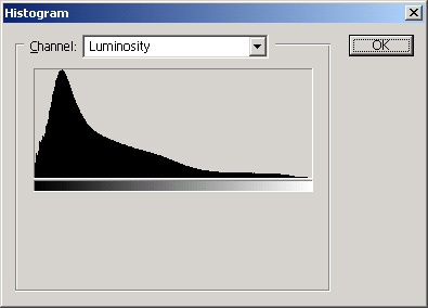
(luminosity). The histogram is displayed as a bar chart. Sometime the chart
looks "spiny", and the shape of the chart can be difficult to analyze.
One side effect of using the bgsmooth
utility is a smoother histogram. Note that a low-resolution image can have
a somewhat different histogram from a high-resolution version of the same
image. For the purposes of this introductory article, the terms luminosity,
brightness
and RGB channel can be taken to be equivalent, although in scientific
contexts, they can have important differences.
 |
 |
| Figure 1a. This histogram of the image shown in Figure 2a is "healthy" and is practically unclipped. | Figure 1b. This histogram (of the image in Figure 2b) is severely clipped on both ends. The dark end is jammed up against the left side of the chart. The bright end runs into the right side, yielding a spike there. |
Clipping
For optimal processing, the histogram should be examined before and after each significant step. One of the most important uses of the histogram is to see if the values are clipped. A histogram that is not clipped has left and right tails that decline to zero before reaching the sides of the chart.Clipping can occur on the dark end (left) of the histogram or on the
bright end (right). Clipping on the left means that too many pixels become
too dark. This makes the left side of the histogram curve "run into" the
left side of the chart. An image clipped on the left will probably have
an excessively dark background. Many of the dimmest features (e.g. delicate
nebulosity) will not be visible to the viewer. Clipping can occur on the
bright end as well. This is usually seen as larger harsher stars or excessively
bright "burned out" areas that obscure the interesting features there.
 |
 |
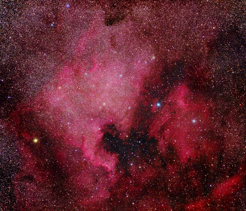
| Figure 2a. This is an unclipped photograph of the North America and Pelican Nebulae in Cygnus by the author. The source was a single 90-minute exposure with a Pentax 67 camera and an Astro-Physics 130 EDF refractor on hypersensitized Kodak PPF 400 film, and it was anti-vignetted. | Figure 2b. This is the same image except that it is clipped it on both the dark end and the bright end. The result is that the background is black and is missing faint nebulosity. The bright areas and stars are "burned out". The image has lost its subtle shading. |
When a processing step clips the histogram, information is lost, and whats worse, no combination of subsequent processing steps can recover that lost information. The only way bring back the information is to revert to a version of the image prior to the step that caused the clipping. With improper parameters, the film scanning process can cause clipping. In that case, the way to get the lost information is to scan again with corrected parameters. A few objects, such as the Great Nebula in Orion, inherently have such a large range of brightness values, that they challenge the dynamic range of the recording medium (e.g. slide film). A good solution is to combine at least two exposures of differing lengths. That technique is covered in the article "Combining Exposures with Layer Masks" by Jerry Lodriguss in January 2001 S&T.
Most photographers process color images in 8-bit RGB Mode. The luminosity of each pixel is a weighted average of the red, green and blue brightness values of the pixel. Four related histograms analyze the red, green, blue, and luminosity channels. A well adjusted image has little or no clipping of any of the four channels.
Are there circumstances when it is appropriate to clip? Yes, as long as you understand what's being traded off. For example, you may have what you consider to be an unattractive background. In that case, if the histogram ends up being clipped on the dark end, that may be fine. In that case, you are intentionally suppressing unwanted information. However, this should be the exception, not the rule. In any case, slight clipping usually is not a problem.
Although clipping is usually bad, the opposite can be bad, too: a histogram with lots of unused space on either side. It is usually desirable for the histogram of a processed image to stretch from near the left side to near the right side (as in Figure 1a). A histogram with lots of unused space indicates a loss of dynamic range. Essentially the image is not taking full advantage of the range of available brightness values. Such an image will have low contrast and will appear "milky" or dull.
Levels
Most image processing software includes a levels tool for directly manipulating the histograms of an image. Levels have their uses, but they are not as powerful as curves. Levels can be used as the first step after scanning or anti-vignetting. In each of the red, green and blue channels, the outer limits can be manually moved to just outside of the ends of the tails. This makes the histogram stretch completely from the left side to the right side, and it usually makes the subsequent curving step easier.Tip: If your film scanner/software has a 16-bit mode, it is simplest to set its parameters "wide" to minimize clipping. Then in Photoshop, adjust the levels, and convert to 8-bit mode. Then add the curves layer.
Curves
Image processing programs like Photoshop provide a Curves dialog that allows the user to adjust the curves of an entire image. Curves are graphical manipulations of the pixel brightness values. In a curves dialog there are four curves corresponding to the histogram channels mentioned above. The curves establish the contrast and color saturation of the image, and they influence the shape of the histograms.Curves provide a brightness input/output function for each channel. The input is represented by the horizontal axis, and the output is represented by the vertical axis. A straight curve that goes from the lower left corner to the upper right corner yields no changes. Lifting a section of a curve essentially raises the output for the various input values, which increases the brightness of the image. Moving the curve to the right reduces the output value of each input value, which makes the image darker. Moving the lower end of the curve to the right makes the background darker. Because the brightness values of the pixels across the image are changed by a curve, the histogram is changed. When the slope of a curve section is made steeper, it increases the contrast of the corresponding pixels.
Curves are easily adjusted by dragging points of the curve with the mouse. Just click on a point of the curve and hold down the left mouse button, then drag the point to the desired location. When Preview is turned on, the effect on the image can be seen immediately as the curve adjustments are made. You can separately adjust the red, green and blue curves, without touching the luminosity (RGB) curve, which provides powerful control over the color balance of the image.
For optimal use of Photoshop (version 5 and up), it is recommended (but not required) that a curves processing step be introduced as a layer. However, the discussion of layers is beyond the scope of this article. It should be noted that unfortunately, Photoshop (up through version 6.0) layers do not support 16-bit channels.
Note that in a Photoshop curves dialog, the horizontal bar with the
two tiny triangles can be clicked, which flips the direction of the input
brightness. This can be confusing. Unless you have a specific need, it
is recommended that the dark end always be oriented to the left, which
is the default.
 |
 |
| Figure 3a. This curve dialog for the red channel avoided clipping the histogram in this case. This nonlinear curve increases midrange contrast and darkens the background. Figures 1a, 2a and 3a correspond to one another. | Figure 3b. This steep straight curve yielded excessive contrast and clipped the histogram. Figures 1b, 2b and 3b correspond to one another. |
Photoshop provides an automatic curves feature. This usually makes an image look much better than its raw form. However, the auto curves are inferior to what can be accomplished manually. Auto curving yields straight curves which tend to clip the image. Optimal curves, which can be achieved manually, are usually nonlinear. The curve shape in Figure 3a is typical. Sometimes complex shapes such as an S-shape are useful. The best way to learn curves is to experiment with the software (e.g. Photoshop) on a raw unclipped image.
The lower ends of the curves establish how the background appears. In general it is best not to make the background a pure black, which clips the image on the dark end. Instead usually the darkest areas of the background should be a very dark gray (e.g. red=20, green=20, blue=20). This allows faint portions of the image to be seen. The pixel levels can be seen in the Photoshop Info Window when the cursor is located over any point of the selected image. Set the Eyedropper "Sample Size" Option to "5 by 5 Average" and test the background at various points around the image.
Sometimes curves by themselves are not enough to present maximum detail in the brightest areas of an image. Unsharp masking is one technique that can be helpful in that case, but that technique is not covered here. Also, it should be noted that curves can be applied to limited portions of an image by using a feathered mask.
Can curves rescue a bad image? Good curves help make any image look its best. But if a raw image fundamentally contains little information, or contains too much noise or too many artifacts, there is simply a limit to how good it can look. However, with a good raw unclipped image, very slight differences in the curves can make large differences in the result. Therefore, if the image appears to be good, take some time to get the curves right. To fully master curves requires practice, patience, and an artists eye.
Vignetting
Typically vignetting is the darkening of an image away from its center. In a raw image it appears as a subtle form of "tunnel vision", but it becomes obvious when its contrast is increased. Virtually all telescopic imaging systems have vignetting. CCD imagers usually eliminate vignetting with flat field processing. Photographers that are inexperienced with digital processing often deal with vignetting by cropping away the outer parts of the image or by ignoring the vignetting. Moderate vignetting can be eliminated by various processing techniques. For further information, see the article "Fixing Vignetting in Astrophotos" by Sean Walker in the September 2001 S&T.The point in mentioning vignetting here is that it will probably result in clipping of the histogram on the dark end. Uncorrected vignetting usually results in loss of information and vanishing of what might have been beautiful faint nebulosity in the outer regions of an image. The anti-vignetting layer should be located underneath the curves layer.
Conclusion
Curving is the single most important technique for digital processing of astronomical images. Curving adjusts contrast, color saturation and color balance. For the casual photographer, curving may be the only processing technique needed. For the serious photographer, curves and histograms must be well understood before more advanced techniques can be mastered. Once an image is successfully curved, it can be printed, emailed, uploaded to the internet, and electronically submitted to publishers.MATT BENDANIEL (
