|
HF
Propagation tutorial
by
Bob Brown, NM7M, Ph.D. from U.C.Berkeley
Propagation
prediction programs (VII)
Now
the past little exercise used old-fashioned tools to do the 5V7A
propagation prediction but at a miserably slow pace. Those really drew on three fundamental ideas - the presence
of F-region ionization, D-region absorption limiting signal
strengths and the geomagnetic field organizing the ionosphere.
So using nothing more than the times of sunrise and sunset,
those concepts gave a qualitative view of propagation.
But without hard numbers, MUFs and signal/noise ratios, that
would never meet the needs of the tough decision-making for a
DXpedition or a DX contest operation. Hopefuly thanks to propagation
prediction programs, we had the opportunity to confirm the opening to
Togo late in the eve.
With
computers brought into the matter, the times of sunrise and sunset
can be calculated with astronomical precision and DX windows found
for working 5V7A on the low bands. The next big problem would be finding the sort of signal
strength that could be expected. So a knowledge of the operating modes or hop structures is
required, primarily a problem in two dimensions, in the plane of the
great-circle path. That sort of thing is done very well by the ray-tracing
in the PropLab Pro
program or using a VOACAP-based
application.
 |
 |
|
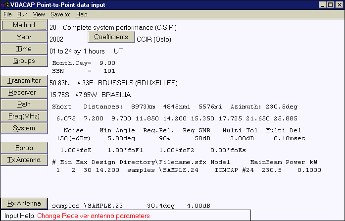
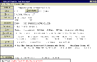
At
left the VOACAP
interface that uses a complex ionospheric model with tens of
functions to predict propagation conditions for a complete
communication circuit using not less than 30 parameters in
input. This prediction is set for a single path between
Brussels (ON) and Brasilia (PY) on September 2002 (SSN =
101, SFI = 146) using a Yagi at the transmitter side with
100 W PEP with a takeoff angle of at least 5°, a dipole at
the receive site and a QRM level of -150 dBW (or S1).
Working in SSB, the S/N required reliability (SNR) is set to
50 dB and the circuit required reliability (SRNxx) to 90%.
At right the forecast predict openings between 7 and 14 MHz with
signal between S3 and S4, thus weak. Other charts (SNR) confirm
the low level of signals with a S/N ratio not higher than 22 dB. Imagine
that 2 years later, in 2004 with an SSN close to 25, conditions
worstened with a gradual closing of upper bands. Currently
only VOACAP-based applications are able to establish
forecasts with such an accuracy. |
|
On
the higher bands, where MUFs, absorption and E-cutoffs are a
concern, computer programs can do a decent job of finding how the
ordinary modes would change in the course of a day, say E-hops
during the day and F-hops at night as well as mixed modes across
sunrise and sunset. But those programs cannot deal with the ionospheric effects from
electron density gradients near the terminator or geomagnetic
equator so certain modes, like chordal hops and ducting, would not
included in their analysis. That's
leaves a gap when it comes to having a complete prediction and so
computers are fast but will not be as fully quantitative as hoped
for in replacing the qualitative efforts used earlier.
As
you might expect, the earliest computer program in amateur use,
MINIMUF, resembled the scheme with ionospheric maps from the
U.S. Dept. of Commerce and just used the control point method for MUFs, via
F-region propagation. Neither signal strength nor noise were considered so the method worked best
at the top of the amateur spectrum and for very high levels of solar
activity. That was unfortunate as amateurs used the same methods at low levels of solar
activity, often with misleading or disappointing results.
But
MINIMUF fired the imagination of many amateurs and various
accessories, including E-layer cutoff calculations, were added to
the original code. For example, MINIPROP Version 1 used the F-layer
model in MINIMUF and had calculations for E-cutoff and signal strength
as well. The early work of Raymond Fricker, MICROMUF 2+ published by
Radio Netherlands, was similar but the E-cutoff was regarded as
giving values for the LUF, the lowest useable frequency. That's not right
as LUF is a D-region matter.
But
there was a basic difference between Fricker's MICROMUF 2+ and
MINIMUF, how the critical frequency information was obtained.
Fricker's F-region algorithm used 13 mathematical functions to
simulate the database for critical frequencies from vertical
sounding while MINIMUF relied on just one function, adjusted to
represent the results of a limited set of oblique soundings.
In
another program released at the same time, IONPRED, one of VOACAP
precursors, Fricker introduced a novel scheme of
hop-testing. Essentially,
the program looked at each hop in detail, at the points where the
E-layer was crossed and at the highest point where the critical
frequency of the F-region was important. So the hop-testing involved
determining whether the mode was reliable by seeing if operating
frequency was above or below the E-cutoff frequency by 5% and less
than the critical frequency for F-region propagation by 5%.
With
an initial choice of radiation angle, the path structure could be
sorted according to E- and F-hops, depending on the outcome of the
tests along the way. Fricker also adjusted the height of the F-region
according to local time so hop lengths were not constant along a path.
As a result, the path could over- or under-shoot the target
QTH. If the error was more than 25 km, another radiation angle was
chosen and the process started again.
|

|
|
All
output parameters that can be displayed in a model like VOACAP for a specified
circuit (using Method 20). |
In IONPRED, Fricker also calculated the ionospheric
absorption, in dB, and added that to the signal loss due to spatial
spreading or attenuation and ground reflections.
Another
innovative feature of IONPRED was the use of availability of the
path, the number of days of the month it would be open for reliable
communication. That was
something like the FOT-MUF-HPF idea discussed earlier but in the
case of IONPRED, the number of days was treated as a continuous
variable in contrast to the upper or lower decile approach with the
FOT-MUF-HPF method.
As a result, the path could over- or under-shoot the target
QTH. If the error was more than 25 km, another radiation angle was
chosen and the process started again.
Nowadays,
the method used by Fricker in IONPRED has been improved upon by the
use of mode-searching in the MINIPROP PLUS program and in all
subsequent applications. Here, the idea is to work up a number of
successful modes and then find the one with the greatest signal
strength. With computer
speeds in the '80s, Fricker's method was extremely time-consuming,
to say the least, but nowadays computer speeds are such that the
whole process of mode-searching takes a second or two! Hopefully
IONPRED was soon corrected, and as you know mutated in IONCAP then
VOACAP.
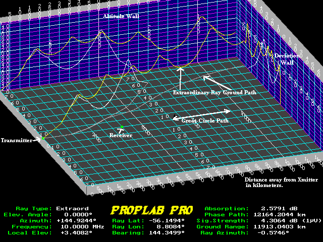
In
a sense, the ray-tracing in PropLab Pro is like hop-testing as it
just goes forward for a given choice of radiation angle and the
calculation stops if the trace is lost to Infinity or stops in the
vicinity of the target QTH. As
you might expect, the main problem with that approach is that the
hops may either fall short or go beyond the target, making it a
slow, iterative process to get the path for RF from point A with
point B. Beside that,
the user would have to evaluate the suitability of the path, whether
the number of E-hops would make it too lossy or otherwise. For that reason, I admire how PropLab Pro goes about a
problem but it's too slow for an impatient person like me.
But
we can use the ray-tracing in the PropLab Pro program to see paths
in both two or three dimensions. It should be said the 2-D case comes fairly close to dealing
with the problem in a proper sense by putting in the appropriate
ionosphere for each hop on the path, considering date, time and SSN.
But it does not take into account terrain, such as the slope
of the ground nor the nature of the reflecting surface. Taking one hop at a time, the calculation does takes into
account the change in height of the ionosphere but not any tilts or
gradients. That is left for the 3-D case.
The
three-dimensional ray-tracing is based on solving equations of
motion for the ray path, just like Newtonian Mechanics finds the
paths of satellites and spacecraft. There are equations for the path advance along and upward in
the great-circle as well as the motion perpendicular to that plane.
The skewing of paths is small in the HF range and thus, it is
usually neglected in ray-tracing. That is because refraction goes
inversely as the square of the frequency and electron density
gradients across paths that occur in the quiet ionosphere are
relatively small. The
exception to that statement is the auroral zones where large
gradients occur.
But
at lower frequencies, like 1.8 MHz in the 160 meter band, the
refraction or bending of paths becomes larger because of the lower
frequency and other effects become important. In particular, the gyration
of ionospheric electrons around the geomagnetic field occurs at a rate
which is comparable to the signal frequency. So
the entire approach to the ionosphere has to be redone, put in more
general terms without any approximations. That complete theory was due to Appleton, is called
magneto-ionic theory and has been around for about 60 years.
Polarization
and RF coupling into the ionosphere
Among
the results of the more general theory are that propagation now
depends on the angle between a ray path and the local magnetic
field; further, the waves which are propagated in the medium are
elliptically polarized, another way of saying they consist of two
components at right angles to each other and which have a phase
difference between them. Beyond
that, there are two modes, with opposite senses of rotation of the
electric field vector, the ordinary and extra-ordinary waves.
The
simple, linearly polarized waves that are so familiar in the
discussion of HF signals are just a limiting case of elliptical
polarization, when one of the two components at right angles has a
very small amplitude compared to the other one. In magneto-ionic
theory, that limiting type of polarization results when signals
are sent perpendicular to the magnetic field. The other case is
circular polarization, when signals are sent along the magnetic
field direction. Then, the two components at right angles are equal in
amplitude and out of phase by 90°.
Those
features of propagation were evident in the early days of
ionospheric sounding as two echoes were returned for each signal
sent upward, the ordinary and extra-ordinary waves, and you will see
them on any ionograms that you may inspect. So magneto-ionic theory is
a part of the reality of radio propagation. But, for
DXers, there is something of a happy simplification as over long
distances, the extra-ordinary wave is heavily absorbed and only the
ordinary wave needs to be considered.
There
is another interesting aspect to propagation down on the 160 meter
band, the coupling of RF into the ionosphere. As you know, there is a polarization to the waves emitted by
an antenna and on 160 meters, vertical antennas are used most often.
That is due to the wavelength being so long that most
horizontal dipoles cannot be placed very high, in terms of
wavelengths, and thus suffer from high radiation angles, being the
so-called "cloud warmers".
|
|
|
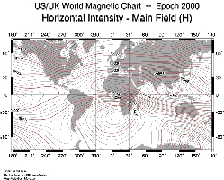
Intensity
of the horizontal component of the geomagnetic field. |
Now
in magneto-ionic theory, the polarization of a wave changes
continously in the ionosphere as it is propagated through the
geomagnetic field. But
there are two limiting polarizations, typically at altitudes around
60 km, where the wave enters the ionosphere near point A and where
it leaves the ionosphere near point B. When worked out in detail, the theory says that there will be
a signal loss, in dB, at entry because of any mismatch between the
wave polarization from the antenna and the limiting (elliptical)
polarization at entry point A.
For
example, signals going in the E-W direction from a vertical antenna
at the equator are poorly coupled into the ionosphere because of the
polarization mismatch, with vertically polarized waves going against
the horizontal field lines. Similarly,
there may be signal loss at the exit point B due to any mismatch
between the limiting polarization on exit from the ionosphere and
the polarization of the antenna at point B.
As
indicated, magneto-ionic theory is quite complicated, with
elliptically polarized waves and all that, but for signals going
from point A to point B, we need not concern ourselves about what
goes on high up in the ionosphere between those two points, only the
antenna types and the limiting polarizations at the endpoints of the
path. That makes life a lot simpler.
Another
point about this frequency range; signals can become trapped in the
electron density valley above the E-region at night. Thus, if they
enter the region, they may be reflected back and forth between the
bottom of the F-region and the lower limit at the top of the E-region. That
means they'll rattle back and forth between those altitude limits
like a ball sliding down a smooth trough. Only if the walls of the
trough change in height can the ball get out or, equivalently, can
signals get out of the duct if the lower ionosphere changes. In
that regard, ducting is undoubtedly responsible for the long-haul
DXing done on 160 meters as it avoids repeated ground reflections
and traversals of the lower ionosphere which absorb signals at a
very high rate.
Reference
Notes
A
review of various propagation programs can be found in the QST
issues for September and October 1996.
Note
by LX4SKY. An updated
list of programs is available on this site, in the next article : Review
of HF propagation analysis and prediction programs, that list not
less than 50 applications.
The
above discussion gives a very brief summary of the principal aspects
of magneto-ionic theory, as it applies to propagation. An analytical summary of the theory is given in Davies'
recent book, Ionospheric
Radio; however, it really requires a strong
background in electromagnetic theory at the level found in
university courses in physics and engineering. It should be noted that the method of the theory has a
broader application as it represents the first steps toward the
study of plasmas in the solar system and in out space.
A
discussion and some quantitative aspects of polarization loss on 160
meters are given in my article in the March/April '98 issue of The
DX Magazine. In addition, a fuller discussion of magneto-ionic theory and 160 meter
DXing is given in Top Band Anthology, published recently by the
Western Washington DX Club.
Radio propagation fundamentals
We
turn now to other aspects of propagation, from predictions to those
circumstances which may disrupt propagation and make predictions go
awry. But in doing that, a bit of history would help chart the
course.
|

|
|
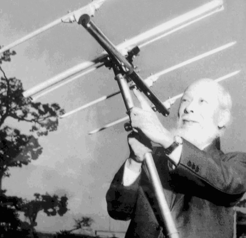
Dr
Hidetsugu Yagi presents his ultimate DXer's gun, the best
antenna design ever made for DXing. Still
another japanese product of quality, Hi ! |
First,
radio is more than 100 years old now
(in 1901 Marconi sent successfully the first wireless message from
England to the U.S.A) and the course of events has been
onward and upward, in frequency and into the ionosphere. Thus, the
earliest signals were down in the kHz region and now technology has
advanced to the point where amateurs are operating in the GHz part
of the spectrum. But it
has been a steady advance in frequency and as we know now, that
means signals going higher and higher into the ionosphere as their
effective vertical frequency increased.
Amateur
operations start in the medium frequency (MF) range with the 160
meter band, around 1.8-2.0 MHz. If one looks into the ray-traces for that band, it is clear
that signals in normal communications circumstances stay below the
200 km level most of the time. Of course, ionospheric absorption on that band is so great
that DX operations are attempted only on paths in full darkness.
Going
to the high frequency (HF) range, 3 - 30 MHz, signals go higher
toward the F-region peak around 300-400 km and darkness becomes less
of a necessity near the top part of the spectrum. In fact, solar
radiation is needed to bring the level of ionization up to the level
required for propagation.
Historically,
in the time that operating frequencies rose, the range of DX
contacts increased and it became apparent that the solar cycle
played a role in propagation. Moreover,
various disturbances became apparent.
So the early '20s had amateurs opening up trans-Atlantic
operations and that was commercialized in the late '20s with the
advent of radiotelephone circuits to Europe. In that time, it was found that the communication links
failed during geomagnetic storms. Those could last for days but there were also strange
blackouts that lasted anywhere from just a few minutes up to an hour.
In 1937, those short wave fadeouts (SWF) were found to be associated with solar
flares. Moreover, it was becoming apparent that the disruptions to magnetic
storming came a day or so AFTER solar flares.
From
all that, it became clear that the sun was a major player in the
field of radio propagation and scientists began looking into the
details. The SWF
problem was fairly simple, just being the release of electrons in
the ionosphere from the photoelectric effect of solar X-rays.
The magnetic storm effect was a more subtle problem as it
implied some slower process, not X-rays moving across the solar
system at the speed of light. In that regard, those geophysicists who studied the earth's
magnetic field proposed that there was a stream of matter sent out
from the sun and then its encounter with the geomagnetic field was
the triggering mechanism. From
the time delays between flares and storms, first estimates were made
of the speed of the solar matter. More than that, they could not say at the
time.
Now
that brings up the question of just how far out geomagnetic field
lines extend from the earth. Of
course, that goes to the model of the geomagnetic field in use at
the time. That was, in simple terms, the sort of thing you get if you
stuff a bar magnet into the earth and look at how the field lines
extend past the surface of the earth. In short, the model back in the
'40s and '50s was that for a
centered dipole field that was tipped with respect to geographic
coordinates, the dipole axis piercing the earth's surface at 79.3° N, 71.8° W
at the north pole and the south pole through the corresponding
antipodal point.
That
was the field used when the first Pioneer space shots took place
after the IGY, an experiment looking at the strength and orientation
of the earth's field as the spacecraft moved out, away from the
earth. That flight
produced a REAL surprise, with data showing the earth's field
varying slowly and in an orderly fashion as the spacecraft moved
outward but then suddenly, when it reached something like 8 earth
radii, the field became weaker and less organized, almost random in
its orientation. Clearly,
the orderly dipole field no longer described the situation at those
distances, giving way to the presence of an interplanetary magnetic
field. And what was previously considered as empty space, except for
meteoritic dust and debris, was also found to contain of plasma
(protons and electrons) that was streaming away from the sun.
Now,
before exploring that extreme, we should look at the dipole field
and see what could be expected from it. As you know, say from your high school physics course, the
field lines pass out of the southern hemisphere and then after going
out some distance, they return and enter the northern hemisphere of
the earth. That was the
classical picture; so let's see what it says, at least until we get
into trouble with the Pioneer data.
Now
the magnetic dipole has a system of coordinates of its own, related
to the direction of its axis relative to the geographic axis and
equatorial plane. With the dipole orientation given above, one can
work out the magnetic coordinates of any point on the earth. For example,
my location at 48.5° N and 122.6° W is one that corresponds to 54.4° N, 62.1° W
in the dipole coordinates. OK?
But
let's look at the dipole and its field lines. They go out from the southern hemisphere and come back down
into the northern hemisphere. But how far do they go out? That
would be important when it comes to thinking about the collision of
solar plasma and the dipole field, suggested by the geomagneticians.
It's not hard to work out where the magnetic field lines
cross the plane of the geomagnetic equator and there is a simple
relation between that distance and the magnetic latitude where the
field lines start:
Ö¯L
= 1 / cos
j
with
j
as the magnetic latitude and L is the distance, measured in
earth radii (Re).
Now
if you conjure up the image of a dipole, surrounded by its magnetic
lines of force, you can see that low-latitude field lines do not go
out very far from the surface of the earth. But it's a different story for high latitude field lines and
if worked out, we obtain the following table :
|
Mag Lat (degs) Distance (L in Re)
10
1.03
20
1.13
30
1.33
40
1.70
50
2.42
60
4.00
70
8.55
80
33.2
|
So
the high latitude field lines are the ones in harm's way when it
comes to the collision between the plasma coming from the sun and
the earth's field. And,
by the same token, the low-latitude field lines that go out only
short distances from the center of the earth are pretty well
protected from the direct effects of the collision between solar
plasma and the geomagnetic field. Of course, that fits with your operating experience, paths
going across the polar cap are far more subject to disruption than
those going to low latitudes.
Before
getting to the nature of the various propagation effects that
originate on the sun, we should note briefly that the view of the
earth's field that I gave in the introduction is not quite
the full story. In
particular, it was suggested that the solar wind blowing by the
obstacle of the geomagnetic field is like the flow problem of a
bullet in air, but now with the bullet (geomagnetic field) fixed and
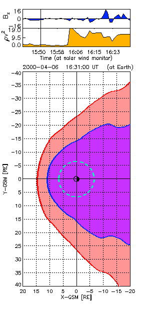
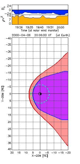
the air (solar wind) in relative motion. So it was suggested (and verified) that a bow shock in the
solar wind was out there in front of the magnetosphere as displayed
at right.
Now,
to carry the aerodynamics a bit further, it was suggested that the
position of the bow shock would vary, moving closer to the earth at
higher speeds of the solar wind.
And that proved to be the case, obtained by satellite
observations after the original work with Pioneer I. But the geomagnetic field is a bit different than a hard
obstacle and it was expected that the field could be compressed at
times, particularly if the solar wind came at it as a sudden blast.
And, as you guessed, that is the case as shown by magnetic sensors on
geostationary satellites. During
some severe magnetic storms, those satellites report conditions
which put them right in the interplanetary magnetic field, showing
that the magnetosphere has been compressed by the solar wind and
that the magnetopause was temporarily inside 6.6 Re. Absolutely amazing!
Now,
having told you about the troubles of geomagnetic field lines, think
back a bit to what I said earlier: they are the things which hold
your precious ionospheric electrons in place! So maybe all those
disruptions in propagation during magnetic storms are not all that
surprising, with field lines being pushed around by the solar wind.
There's
more to magnetic storm effects than just compressing the field lines
in front of the earth. As I suggested way back in the second
page, field lines on the front of the magnetosphere can be dragged into the magnetotail.
In that process, the ionospheric electrons of the F-region on
those field lines are removed from the front of the magnetosphere
and, in essence, are distributed on much longer field lines on the
rear of the magneto-sphere. On
both counts, the high-latitude F-region suffers a loss in ionization
and critical frequencies in the affected regions are reduced. Of course,
the sun shines, day in and day out, so with some
magnetic quiet, solar illumination will restore the regions and
communications across those high latitudes returns to normal.
Those
words of explanation will have to suffice as the problems of the
magnetosphere are quite complicated, with unfamiliar or
non-classical ideas, and are best left for the magnetospheric
physics-types to wrestle with. We need not get enmeshed in the
details, only be able to recognize when there's a problem and
consequences that will follow. In that regard, the records of magnetometers at high
latitudes are our best bet as they give vivid portrayals of the
storms that develop, thanks to simultaneous, yet secondary effects
which result. There, I
am thinking of the aurora, both optical and radio, as well as the
current systems which build up during a disturbance initiated by the
solar wind.
Again,
the details need not concern us but the main features are what we
note: optical emissions coming from above the 100 km layer, VHF
reflections off of auroral displays, ionospheric absorption of
signals going across an active auroral zone and strong magnetic
disturbances observed on the ground from the current systems which
develop along the ionized region. More on this in the the last
chapter.
Research
Notes
A
good historical account of the early days of radio can be found in
the first chapter of McNamara's book, "Radio Amateurs Guide to
the Ionosphere" published by Krieger Publ.Corp. in 1994. And
it's a good book too. Get a copy if you are serious about radio propagation.
Add
also the link to this web pages, History of
amateur radio, appreciated by ARRL's staff and CQ Magazine's
editors too.
Last
chapter
Geomagnetic
disturbances
|